We often summarize that the fiscal theory is a theory of the price level: The price level adjusts so that the real value of government debt equals the present value of surpluses. That characterization seems to leave it to a secondary role. But with any even tiny price stickiness, fiscal theory is really a fiscal theory of inflation. The following two parables should make the point, and are a good starting point for understanding what fiscal theory is really all about. This point is somewhat buried in Chapter 5.7 of Fiscal Theory of the Price Level.
Start with the response of the economy to a one-time fiscal shock, a 1% unexpected decline in the sum of current and expected future surpluses, with no change in interest rate, at time 0. The model is below, but today's point is intuition, not staring at equations. This is the continuous-time version of the model, which clarifies the intuitive points.
 |
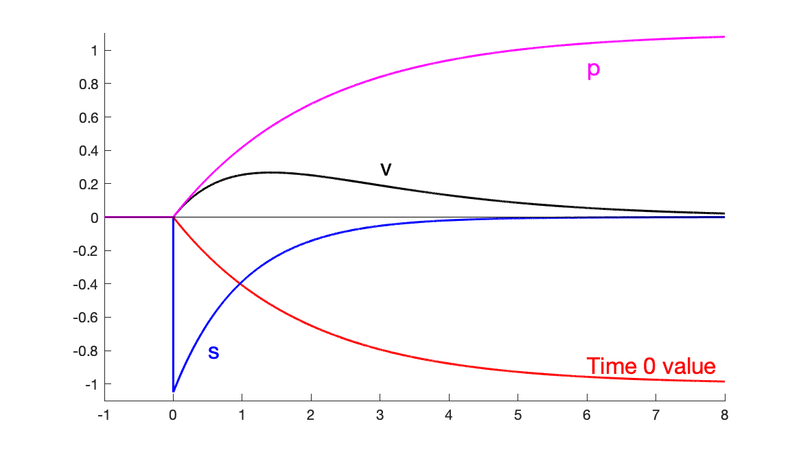
| Response to 1% fiscal shock at time 0 with no change in interest rates |
The one-time fiscal shock produces a protracted inflation. The price level does not move at all on the date of the shock. Bondholders lose value from an extended period of negative real interest rates -- nominal interest rates below inflation.
What's going on? The government debt valuation equation with instantaneous debt and with perfect foresight is \[V_{t}=\frac{B_{t}}{P_{t}}=\int_{\tau=t}^{\infty}e^{-\int_{w=t}^{\tau}\left( i_{w}-\pi_{w}\right) dw}s_{\tau}d\tau\] where \(B\) is the nominal amount of debt, \(P\) is the price level, \(i\) is the interest rate \(\pi\) is inflation and \(s\) are real primary surpluses. We discount at the real interest rate \(i-\pi\). We can use this valuation equation to understand variables before and after a one-time probability zero "MIT shock."
With flexible prices, we have a constant real interest rate, so \(i_w-\pi_w\). Thus if there is a downward jump in \(\int_{\tau=t}^{\infty}e^{-r \tau}s_{\tau}d\tau\), as I assumed to make the plot, then there must be an upward jump in the price level \(P_t\), to devalue outstanding debt. (Similarly, a diffusion component to surpluses must be matched by a diffusion component in the price level.) The initial price level adjusts so that the real value of debt equals the present value of surpluses. This is the standard understanding of the fiscal theory of the price level. Short-term debt holders cannot be made to lose from expected future inflation.
But that's not how the simulation in the figure works, with sticky prices. Since now both \(B_t\) and \(P_t\) on the left hand side of the government debt valuation equation cannot jump, the left-hand side itself cannot jump. Instead, the government debt valuation equation determines which path of inflation \(\{\pi_w\}\) which, with the fixed nominal interest rate \(i_w\), generates just enough lower real interest rates \(\{i_w-\pi_w\}\) so that the lower discount rate just offsets the lower surplus. Short-term bondholders lose value as their debt is slowly inflated away during the period of low real interest rates, not in an instantanoues price level jump.
In this sticky-price model, the price level cannot jump or diffuse because only an infinitesimal fraction of firms can change their price at any instant in time. The price level is continuous and differentiable. The inflation rate can jump or diffuse, and it does so here; the price level starts rising. As we reduce price stickiness, the price level rise happens faster, and smoothly approaches the limit of a price-level jump for flexible prices.
In short, fiscal theory does not operate by changing the initial price level. Fiscal theory determines the path of the inflation rate. It really is a fiscal theory of inflation, of real interest rate determination.
The frictionless model remains a guide to how the sticky price model behaves in the long run. In the frictionless model, monetary policy sets expected inflation via \(i_t = r+E_t \pi_{t+1}\) or \(i_t = r+\pi_t\), while fiscal policy sets unexpected inflation \(\pi_{t+1}-E_t\pi_{t+1}\) or \(dp_t/p_t-E_t dp_t/p_t\). In the long run of my simulation, the price level does inexorably rise to devalue debt, and the interest rate determines the long-run expected inflation. But this long-run characterization does not provide useful intuition for the higher frequency path, which is what we typically want to interpret and analyze.
It is a better characterization of these dynamics that monetary policy---the nominal interest rate---determines a set of equilibrium inflation paths, and fiscal policy determines which one of these paths is the overall equilibrium, inflating away just enough initial debt to match the decline in surpluses.
 |
| Response to 1% deficit shock at time 0 with no change in interest rate |
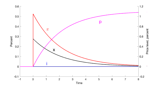
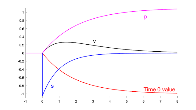
This second graph gives a bit more detail of the fiscal-shock simulation, plotting the primary surplus \(s\), the value of debt \(v\), and the price level \(p\). The surplus follows an AR(1). The persistence of that AR(1) is irrelevant to the inflation path. All that matters is the initial shock to the discounted stream of surpluses. (I make a big fuss in FTPL that you should not use AR(1) surplus process to match fiscal data, since most fiscal shocks have an s-shaped response, in which deficits correspond to larger surpluses. However, it is still useful to use an AR(1) to study how the economy responds to that component of the fiscal shock that is not repaid.)
To see how initial bondholders end up financing the deficits, track the value of those bondholders' investment, not the overall value of debt. The latter includes debt sales that finance deficits. The real value of a bond investment held at time 0, \(\hat{v}\), follows \[d \hat{v}_t = (r \hat{v}_t + i_t - \pi_t)dt. \] I plot the time-zero value of this portfolio, \[e^{-rt} \hat{v}_t.\] As you can see this value smoothly declines to -1%. This is the quantity that matches the 1% by which surpluses decline. (I picked the initial surplus shock \(d\varepsilon_{s,t}=1/(r+\eta_s)\) so that \(\int_{\tau=0}^\infty e^{-r\tau}\tilde{s}_t d\tau =-1.\) )
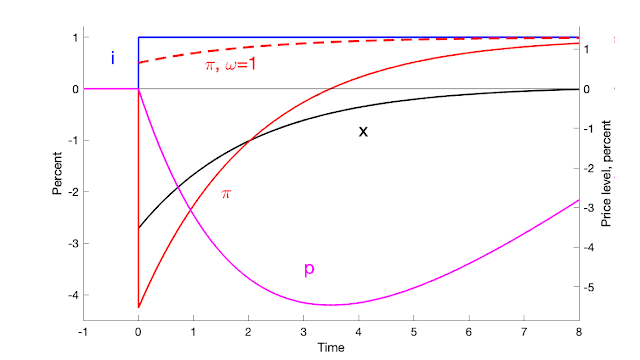 |
| Response to interest rate shock at time 0 with no change in surpluses |
The third graph presents the response to an unexpected permanent rise in interest rate. With long-term debt, inflation initially declines. The Fed can use this temporary decline to offset some fiscal inflation. Inflation eventually rises to meet the interest rates. Most interest rate rises are not permanent, so we do not often see this long-run stability or neutrality property. The initial decline in interest rates comes in this model from long-term debt. As the dashed line shows, with shorter-maturity debt inflation rises right away. With instantaneous debt, inflation follows the interest rate exactly.
Again, in this continuous-time model the price level does not move instantly. The higher interest rate sets off a period of lower inflation, not a price-level drop.
With long-term debt the perfect-foresight valuation equation is \[V_{t}=\frac{Q_tB_{t}}{P_{t}}=\int_{\tau=t}^{\infty}e^{-\int_{w=t}^{\tau}\left( i_{w}-\pi_{w}\right) dw}s_{\tau}d\tau. \] where \(Q_t\) is the nominal price of long-term government debt. Now, with flexible prices, the real rate is fixed \(i_w=\pi_w\). With no change in surplus \(\{s_\tau\}\), the right hand side cannot change. Inflation \(\{\pi_w\}\) then simply follows the AR(1) pattern of the interest rate. However, the higher nominal interest rates induce a downward jump or diffusion in the bond price \(Q_t\). With \(B_t\) predetermined, there must be a downward jump or diffusion in the price level \(P_t\). In this way, even with flexible prices, with long-term debt we can see an instant in which higher interest rates lower inflation before ``long run'' neutrality kicks in.
How does the price level not jump or diffuse with sticky prices? Now \(B_t\) and \(P_t\) are predetermined on the left hand side of the valuation equation. Higher nominal interest rates \(\{i_w\}\) still drive a downward jump or diffusion in the bond price \(Q_t\). With no change in \(s_\tau\), a spread \(i_w-\pi_w\) must open up to match the downward jump in bond price \(Q_t\), which is what we see in the simulation. Rather than an instant downward jump in price level, there is instead a long period of low inflation, of slow price level decline, followed by a gradual increase in inflation.
Again, the frictionless model does provide intuition for the long-run behavior of the simulation. The three year decline in price level is reminiscent of the downward jump; the eventual rise of inflation to match the interest rate is reminiscent of the immediate rise in inflation. But again, in the actual dynamics we really have a theory of \emph{inflation}, not a theory of the \emph{price level}, as on impact the price level does not jump at all. Again, the valuation equation generates a path of inflation, of the real interest rate, not a change in the value of the initial price level.
The general lessons of these two simple exercises remain:
Both monetary and fiscal policy drive inflation. Inflation is not always and everywhere a monetary phenomenon, but neither is it always and everywhere fiscal.
In the long run, monetary policy completely determines the expected price level. As the inflation rate ends up matching the interest rate, inflation will go wherever the Fed sends it. If the interest rate went below zero (these are deviations from steady state, so that is possible), it would drag inflation down with it, and the price level would decline in the long run.
One can view the current situation as the lasting effect of a fiscal shock, as in the first graph. One can view the Fed's option to restrain inflation as the ability to add the dynamics of the second graph.
Don't be too put off by the simple AR(1) dynamics. First, these are responses to a single, one-time shock. Historical episodes usually have multiple shocks. Especially when we pick an episode ex-post based on high inflation, it is likely that inflation came from several shocks in a row, not a one-time shock. Second, it is relatively easy to add hump-shaped dynamics to these sorts of responses, by standard devices such as habit persistence preferences or capital accumulation with adjustment costs. Also, full models have additional structural shocks, to the IS or Phillips curves here for example. We analyze history with responses to those shocks as well, with policy rules that react to inflation, output, debt, etc.
The model I use for these simple simulations is a simplified version of the model presented in FTPL 5.7.
$$\begin{aligned}E_t dx_{t} & =\sigma(i_{t}-\pi_{t})dt \\E_t d\pi_{t} & =\left( \rho\pi_{t}-\kappa x_{t}\right) dt\ \\ dp_{t} & =\pi_{t}dt \\ E_t dq_{t} & =\left[ \left( r+\omega\right) q_{t}+i_{t}\right] dt \\ dv_{t} & =\left( rv_{t}+i_{t}-\pi_{t}-\tilde{s}_{t}\right) dt+(dq_t - E_t dq_t) \\ d \tilde{s}_{t} & = -\eta_{s}\tilde{s}_{t}+d\varepsilon_{s,t} \\ di_{t} & = -\eta_{i}i_t+d\varepsilon_{i,t}. \end{aligned}$$
I use parameters \(\kappa = 1\), \(\sigma = 0.25\), \(r = 0.05\), \(\rho = 0.05\), \(\omega=0.05\), picked to make the graphs look pretty. \(x\) is output gap, \(i\) is nominal interest rate, \(\pi\) is inflation, \(p\) is price level, \(q\) is the price of the government bond portfolio, \(\omega\) captures a geometric structure of government debt, with face value at maturity \(j\) declining at \(e^{-\omega j}\), \(v\) is the real value of government debt, \(\tilde{s}\) is the real primary surplus scaled by the steady state value of debt, and the remaining symbols are parameters.
Thanks much to Tim Taylor and Eric Leeper for conversations that prompted this distillation, along with evolving talks.