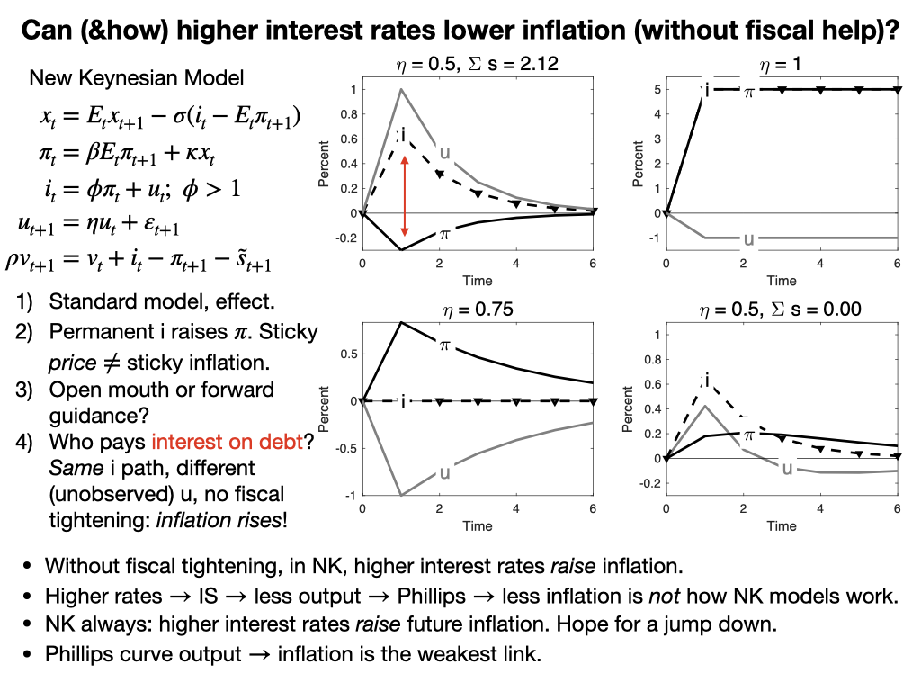
The equations are the utterly standard new-Keynesian model. The last equation tracks the evolution of the real value of the debt, which is usually in the footnotes of that model.
OK, top right, the standard result. There is a positive but temporary shock to the monetary policy rule, u. Interest rates go up and then slowly revert. Inflation goes down. Hooray. (Output also goes down, as the Phillips Curve insists.)
The next graph should give you pause on just how you interpreted the first one. What if the interest rate goes up persistently? Inflation rises, suddenly and completely matching the rise in interest rate! Yet prices are quite sticky -- k = 0.1 here. Here I drove the persistence all the way to 1, but that's not crucial. With any persistence above 0.75, higher interest rates give rise to higher inflation.
What's going on? Prices are sticky, but inflation is not sticky. In the Calvo model only a few firms can change price in any instant, but they change by a large amount, so the rate of inflation can jump up instantly just as it does. I think a lot of intuition wants inflation to be sticky, so that inflation can slowly pick up after a shock. That's how it seems to work in the world, but sticky prices do not deliver that result. Hence, the real interest rate doesn't change at all in response to this persistent rise in nominal interest rates. Now maybe inflation is sticky, costs apply to the derivative not the level, but absolutely none of the immense literature on price stickiness considers that possibility or how in the world it might be true, at least as far as I know. Let me know if I'm wrong. At a minimum, I hope I have started to undermine your faith that we all have easy textbook models in which higher interest rates reliably lower inflation.
(Yes, the shock is negative. Look at the Taylor rule. This happens a lot in these models, another reason you might worry. The shock can go in a different direction from observed interest rates.)
Panel 3 lowers the persistence of the shock to a cleverly chosen 0.75. Now (with sigma=1, kappa=0.1, phi= 1.2), inflation now moves with no change in interest rate at all. The Fed merely announces the shock and inflation jumps all on its own. I call this "equilibrium selection policy" or "open mouth policy." You can regard this as a feature or a bug. If you believe this model, the Fed can move inflation just by making speeches! You can regard this as powerful "forward guidance." Or you can regard it as nuts. In any case, if you thought that the Fed's mechanism for lowering inflation is to raise nominal interest rates, inflation is sticky, real rates rise, output falls and inflation falls, well here is another case in which the standard model says something else entirely.
Panel 4 is of course my main hobby horse these days. I tee up the question in Panel 1 with the red line. In that panel, the nominal interest are is higher than the expected inflation rate. The real interest rate is positive. The costs of servicing the debt have risen. That's a serious effect nowadays. With 100% debt/GDP each 1% higher real rate is 1% of GDP more deficit, $250 billion dollars per year. Somebody has to pay that sooner or later. This "monetary policy" comes with a fiscal tightening. You'll see that in the footnotes of good new-Keynesian models: lump sum taxes come along to pay higher interest costs on the debt.
Now imagine Jay Powell comes knocking to Congress in the middle of a knock-down drag-out fight over spending and the debt limit, and says "oh, we're going to raise rates 4 percentage points. We need you to raise taxes or cut spending by $1 trillion to pay those extra interest costs on the debt." A laugh might be the polite answer.
So, in the last graph, I ask, what happens if the Fed raises interest rates and fiscal policy refuses to raise taxes or cut spending? In the new-Keynesian model there is not a 1-1 mapping between the shock (u) process and interest rates. Many different u produce the same i. So, I ask the model, "choose a u process that produces exactly the same interest rate as in the top left panel, but needs no additional fiscal surpluses." Declines in interest costs of the debt (inflation above interest rates) and devaluation of debt by period 1 inflation must match rises in interest costs on the debt (inflation below interest rates). The bottom right panel gives the answer to this question.
Review: Same interest rate, no fiscal help? Inflation rises. In this very standard new-Keynesian model, higher interest rates without a concurrent fiscal tightening raise inflation, immediately and persistently.
Fans will know of the long-term debt extension that solves this problem, and I've plugged that solution before (see the "Expectations" paper above).
The point today: The statement that we have easy simple well understood textbook models, that capture the standard intuition -- higher nominal rates with sticky prices mean higher real rates, those lower output and lower inflation -- is simply not true. The standard model behaves very differently than you think it does. It's amazing how after 30 years of playing with these simple equations, verbal intuition and the equations remain so far apart.
The last two bullet points emphasize two other aspects of the intuition vs model separation. Notice that even in the top left graph, higher interest rates (and lower output) come with rising inflation. At best the higher rate causes a sudden jump down in inflation -- prices, not inflation, are sticky even in the top left graph -- but then inflation steadily rises. Not even in the top left graph do higher rates send future inflation lower than current inflation. Widespread intuition goes the other way.
In all this theorizing, the Phillips Curve strikes me as the weak link. The Fed and common intuition make the Phillips Curve causal: higher rates cause lower output cause lower inflation. The original Phillips Curve was just a correlation, and Lucas 1972 thought of causality the other way: higher inflation fools people temporarily to producing more.
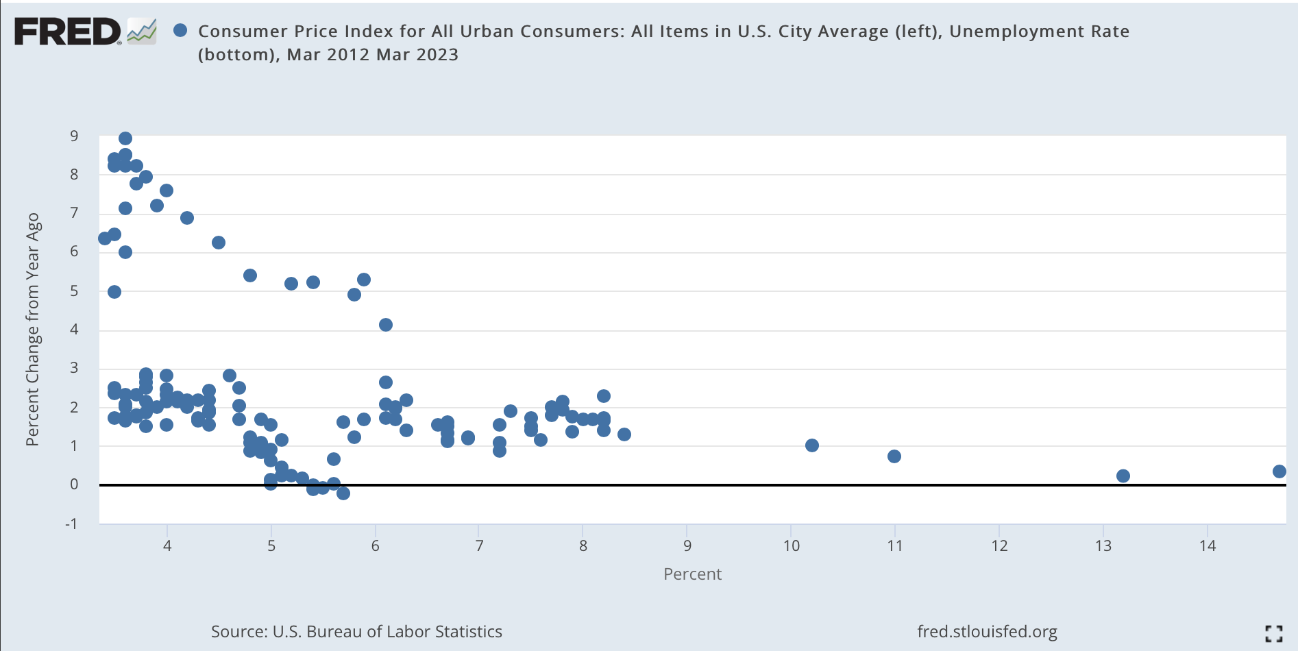
Here is the Phillips curve (unemployment x axis, inflation y axis) from 2012 through last month. The dots on the lower branch are the pre-covid curve, "flat" as common wisdom proclaimed. Inflation was still 2% with unemployment 3.5% on the eve of the pandemic. The upper branch is the more recent experience.
I think this plot makes some sense of the Fed's colossal failure to see inflation coming, or to perceive it once the dragon was inside the outer wall and breathing fire at the inner gate. If you believe in a Phillips Curve, causal from unemployment (or "labor market conditions") to inflation, and you last saw 3.5% unemployment with 2% inflation in February 2021, the 6% unemployment of March 2021 is going to make you totally ignore any inflation blips that come along. Surely, until we get well past 3.5% unemployment again, there's nothing to worry about. Well, that was wrong. The curve "shifted" if there is a curve at all.
But what to put in its place? Good question.
Update:
Lots of commenters and correspondents want other Phillips Curves. I've been influenced by a number of papers, especially "New Pricing Models, Same Old Phillips Curves?" by Adrien Auclert, Rodolfo Rigato, Matthew Rognlie, and Ludwig Straub, and "Price Rigidity: Microeconomic Evidence and Macroeconomic Implications" by Emi Nakamura and Jón Steinsson, that lots of different micro foundations all end up looking about the same. Both are great papers. Adding lags seems easy, but it's not that simple unless you overturn the forward looking eigenvalues of the system; "Expectations and the neutrality of interest rates" goes on in that way. Adding a lag without changing the system eigenvalue doesn't work.
If I am not mistaken, Rotemberg pricing (quadratic adjustment costs) limits the inflation as each firm want to have a lot of small adjustments to limit the cost paid each period.
ReplyDeleteIn continuous time, it's pretty clear that the firm control the inflation rate, with convex costs in inflation, subject to the law of motion of its state that is the price charged.
Actually 'prices sticky' = 'inflation sticky' is a feature of any model with strategic complementarity in pricing, which is true for certain parameter values and appears to be pretty realistic.
DeleteMy question is: what is the transmission mechanism between bank balance sheets and the real economy? The new Keynesian models do not realistically model balance sheets and (in their dynamic stochastic general equilibrium model form) they are actually solved as perturbations around a minimised Lagrangian, so implicitly assume that base minimum is stable in reality. In practice, balance sheets (and other major dislocations, e.g. Ukraine through the price of energy, possibly) may change that underlying minimum.
ReplyDeletevery well said. BTW...not just any Bank...Politically connected banks...like SVB, etc
DeleteCurrently there is about $120,000 of Federal Debt per American
ReplyDeleteInterest Rate...just part of the story!
Is this about dynamic elastities in the end? Maybe I'm confused. Ha
ReplyDeleteThis comment has been removed by the author.
ReplyDeleteThank you for your blog Dr. Cochrane. I am not a professional economist but I believe that the practical application of your theory is ongoing in Argentina, specially for the last two years. In part, I've just found the academic answer of the reality in our country, where specially applies your conclusion.
ReplyDeleteit seems like you're moving i exogenously and deriving u as the endogenous response, isn't that backwards?
ReplyDeleteIn panel 3 and 4 I reverse-engineer the exogenous u that produces a desired endogenous i. That's slightly but crucially different.
Delete
ReplyDeleteOn the Phillips Curve:
The paper by Auclert et al. presumes that the firms determine their product line price changes by calculating the discounted infinite sum of the forward marginal cost of production { mc(t + k∙Δt) } , k = 1, 2, ..., ∞. One who has pursued a career in industry in production and corporate planning executive positions, rather than academia, would not regard that model as practicable for determining the price revisions in response to changes in the economic and competitive environment. Nor would labor inputs be the sole basis for determining marginal cost except in service sectors where labor is effectively the only input factor. Consider, for example, the price of electrolytic copper (an input factor in electric motors), the labor component of the cost is not significant compared to the cost of the raw material and the semi-finished intermediate product, copper wire the processing of which is highly automated and energy intensive rather than labor intensive.
The paper by Nakamura and Steinsson highlights the problem of determining a single parameter value for a multi-sector economy. The difficulty in reducing the data to a single index value which is a function of the state of the economy at any one point in time remains daunting for the economic modeler. This is esp. so when one attempts to remain faithful to the "micro-economic foundations" in the macro model environment.
Towards that end, it is important to revisit the macro model foundational Euler equations and the assumptions used to develop those equations. It will then be seen that the only available alternative to the Calvo- or Taylor- 'sticky price' fixed parameter value, kappa, is to allow kappa to be a state-dependent variable in the model, and accept that the label "Phillips Curve" is a misnomer of no importance. Then write the NK-PC equation as πₜ = β ∙ πᵉₜ + κ(xᵉₜ ,πᵉₜ) ∙ xₜ . The model with this adjustment is no longer linear, but that is neither here nor there because the method of solution is numerical rather than analytical in all but the simplest stripped down versions of the NK-DSGE models currently in use. Identification of the functional relation of κ(xᵉₜ ,πᵉₜ) to the state variables then becomes the challenge for the modeller.
For a view on the history of the Phillips Curve, its origin, its failure, and the hold it has on the current and former chairs of the FRB see James A. Dorn, "The Phillips Curve: A Poor Guide for Monetary Policy", Cato Institute, Winter 2020, here: https://www.cato.org/cato-journal/winter-2020/phillips-curve-poor-guide-monetary-policy#references .
DeleteJohn poses the question: "But what to put in its [NK-PC] place? Good question."
DeleteRoger Farmer and Giovanni Nicolò (both at UCLA) developed a NK-DSGE model that does not include the NK Phillips curve equation in the specification. In place of the NK-PC they substitute what they refer to as a "belief relation" which they describe as a Martingale process represented by the equation E{x(t+1)} = x(t), where x(t) is a state variable. In support of their model, they examine the fit of the NK-DSGE model that includes a NK-PC equation against the same NK-DSGE model with the NK-PC replaced by their "belief relation". The data series examined is USA macro stats from 1954-Q3 to c.a. 2007-Q4.
One would ideally like to have confirmation by extending the econometric analysis through 2022-Q4.
Their paper is freely available from NBER, and R. Farmer's blog site.
"Keynesian Economics without the Phillips Curve",
Roger E.A. Farmer and Giovanni Nicolò, NBER Working Paper No. 23837 September 2017 JEL No. E0,E12,E52
From the conclusion:
"The FM model gives a very different explanation of the relationship between inflation, the output gap and the federal funds rate from the conventional NK approach. It is a model where demand and supply shocks may have permanent effects on employment and inflation and our empirical findings demonstrate that this model fits the data better than the NK alternative. The improved empirical performance of the FM model stems from its ability to account for persistent movements in the data. In the FM model, beliefs about nominal income growth are fundamentals of the economy. Beliefs select the equilibrium that prevails in the long-run and monetary policy chooses to allocate shocks to permanent changes in inflation expectations or permanent deviations of output from its trend growth path. Our findings have implications for the theory and practice of monetary policy. Central bankers use the concept of a time-varying natural rate of unemployment before deciding when and if to raise the nominal interest rate. The difficulty of estimating the natural rate arises, in practice, because the economy displays no tendency to return to its natural rate. That fact has led to much recent skepticism about the usefulness of the Phillips curve in policy analysis. Although we are sympathetic to the Keynesian idea that aggregate demand determines employment, we have shown in this paper that it is possible to construct a ‘Keynesian economics’ without the Phillips curve." © 2017 by Roger E.A. Farmer and Giovanni Nicolò
On Modelling via Computer Simulation:
ReplyDeleteWhen one creates a simulation model based on the NK-DSGE equations above and uses reasonable values for the parameters appearing in those equations (following the text of the blog article) and substitutes for the conditional expectations of the one-period ahead output gap and rate of inflation {xᵉₜ , πᵉₜ} the representation set { xₜ₊₁ + ξₜ , πₜ₊₁ + ζₜ } (where {ξₜ , ζₜ } are the forecasting errors presumed to be stochastic and modelled as random variables with means not necessarily zero), one inevitably finds that the model output is structurally determined by the model construction. The model’s output is influenced by the stochastic variables { ξₜ , ζₜ , εₜ , s͂ₜ }.
The innovations, εₜ , and s͂ₜ , are partly, if not wholly, under the modeller's control (see for example, the discussion of panel 4 above). It should therefore not be surprising to find that the state variable outputs represented in panels 1 thru 4, above, are largely determined by choices made for the time series { εₜ } t = 1, 2, ..., 6.
The Taylor Rule equation, iₜ = φ ∙ πₜ + uₜ , along with the innovation process, uₜ = η∙uₜ₋₁ + εₜ , largely accounts for the behavior displayed in each panel.
On the Fiscal Theory of the Price Level and NK-DSGE models:
The innovation {s͂ₜ} only influences the bond valuation state variable, vₜ . This reflects the absence of money in the NK-IS and NK-PC equations, according to critics of NK-DSGE models. It begs the question: How might {s͂ₜ} be worked into either or both of the NK-IS and NK-PC equations in the model in order to achieve integration of fiscal and monetary policy choices?
If the price level be dependent on the time series {s͂ₜ} and the initial stock of government securities, B₀, and changes in price level determine the rate of inflation { πᵉₜ} via the definition πₜ ≝ d(ln(pₜ))/dt, then it would seem possible to improve the NK-DSGE model by changing either the NK-IS or the NK-PC equations to reflect that dependency. Clearly, the NK-PC equation is the likely starting point.
At the Jan Mayen Arctic weather station, located on a desolate volcanic island 600 miles west of Norway's North Cape and subject to brutal winters, a sign greets visitors. Written in Norwegian, the sign reads "Theory is when you understand everything, but nothing works. Practice is when everything works but nobody understands why. At this station, theory and practice are united, so nothing works, and nobody understands why." -- "Fed Up, An Insider's Take on Why The Federal Reserve is Bad for America", p. 224, Danielle DiMartino Booth, New York, NY, Penguin Random House, 2017.
DeleteYou say: "What if the interest rate goes up persistently? Inflation rises, suddenly and completely matching the rise in interest rate!"
ReplyDeleteBut how could it be that an inflationary tax at 4%p.a. would yield to the government the same revenue as a 2% inflation (I assume that for the rest of the public debt, real interest rates are the same for both inflation rates scenarios)
The rate of inflation that maximizes revenue from the inflation tax is the rate at which the inflation elasticity of money demzz as be is -1, assuming no effect on GDP. James Cover
DeleteThere are countervailing forces at work. A rise in interest rates increases the velocity of circulation. But a rise in rates causes saver-holders to shift their deposits, to increase their precautionary holdings destroying velocity. Ultimately, increased costs make borrowing prohibitive.
ReplyDeleteBtw, you take 'unchanged fiscal policy' to mean unchanged real surpluses. Is that what it should really mean? With proportional taxes higher inflation raises nominal tax receipts, so real tax receipts are unchanged. However, the US budget I believe specifies nominal expenditures, not real. (We say 'we're spending $Xm on education', not 'we are buying Y hours of teaching'). Together this means a higher price level raises real surpluses. Is this not correct?
ReplyDeleteYes, that was sloppy. Here I mean no change in surpluses. FTPL has simulations with fiscal policy rules in which it means no change in residual of those rules.
DeleteA model should be a tool or a servant for the economist. The economist should not be a servant of the model. The only way to keep interest rates low is by putting a flow of additional liquidity into the economy, which eventually must increase the rate of decline in the value of money. Likewise the opposite requires reducing the flow of additional liquidity into the economy. You cannot model inflation without modeling the interaction between liquidity and the real economy. BTW, the only way to increase the amount of liquidity if it is increased by borrowing to to get people to borrow more, i.e., by lowering the nominal rate of interest—unless it is done by helicopter money—which the US government essentidid with stimulus payments.
ReplyDeleteA paper published during the summer of 2008 provides a survey of the NK Phillips Curve ("NK-PC") and the identification issues relating to that model of the interaction between the rate of inflation, the output gap or marginal cost, and monetary shocks.
ReplyDeleteSchorfheide, Frank, DSGE Model-Based Estimation of the New Keynesian Phillips Curve (2008). FRB Richmond Economic Quarterly, Vol. 94, No. 4, Fall 2008, pp. 397-433, Available at SSRN: https://ssrn.com/abstract=2187864
ABSTRACT: "This paper surveys estimates of New Keynesian Phillips curve (NKPC) parameters that have been obtained by fitting fully specified dynamic stochastic general equilibrium (DSGE) models to U.S. data. We examine various sources of identification in the context of a simple analytical model. DSGE model-based NKPC estimates tend to be fragile and sensitive to the model specification, in particular if marginal costs are treated as an unobserved variable. Estimates of the NKPC slope lie between 0 and 4. If the observations span the labor share, which is in most instances the model-implied measure of marginal costs, then the slope estimates fall into a much narrower range of 0.005 to 0.135. No consensus has emerged with respect to the importance of lagged inflation in the Phillips curve."
The article by J. K. Galbraith (U. Texas at Houston) examines inflation, unemployment and actions of the FRB's FOMC in light of the recent developments since the onset of the 2020-21 pandemic in the U.S.
ReplyDeleteJames K. Galbraith, "The Quasi-Inflation of 2021-2022: A Case of Bad Analysis and Worse Response", FEB 2, 2023
This essay is forthcoming in the Review of Keynesian Economics.
https://www.ineteconomics.org/perspectives/blog/the-quasi-inflation-of-2021-2022-a-case-of-bad-analysis-and-worse-response
Observation and conclusion:
"Third, there is the effect of higher interest rates on business costs. Interest, after all, must be paid. Sooner or later, the higher short-term rates will bleed into the accounts of business borrowers, and some of the effect will be passed along, so far as conditions permit, to their customers. To that degree, a tight monetary policy is inflationary before it is disinflationary.
"9. Conclusion
"In sum, the theoretical construct of pure inflation is of no use in understanding the price events of 2021 and 2022 in the United States. By extension, the conventional tools of the Phillips Curve, NAIRU, potential output, and money-supply growth are equally useless. By further extension, the “anti-inflation” policies of the Federal Reserve have acted on asset markets (which are not part of theoretical inflation) while taking credit for the end to a price process in produced goods that was transitory in any event. Yet the Federal Reserve is now stuck in a posture guaranteed to destabilize economic activity sooner or later, while the economy remains vulnerable to additional potential price shocks emanating from the same sources already seen, including real resources, supply chains, wars, pandemics, and the policies of the Federal Reserve itself. These can be dealt with, if at all, only by policies in each specific area."
Have you read this post from Neil Wilson on interest/price spiral:
ReplyDeletehttps://new-wayland.com/blog/interest-price-spiral/
The Myth
The standard line is this from the Bank of England
“when we raise Bank Rate, banks will usually increase how much they charge on loans and the interest they offer on savings. This tends to discourage businesses from taking out loans to finance investment, and to encourage people to save rather than spend.”
“Overall if loans go down, financial savings must go down by exactly the same amount.
If you want the stock of bank loans to come down, while the stock of bank deposits goes up, then, unfortunately, reality won’t let you do that.”
“the cost of credit is incorporated into the cost of all goods and services. The higher the interest rate, the higher the price.
The Myth recommends pouring fuel on the fire. MMT recommends a permanently zero Bank Rate, and making central bankers, along with their expensive entourage, redundant.”
Question to you do you support permanent ZIRP?
"...higher interest rates without a concurrent fiscal tightening raise inflation, immediately and persistently."
ReplyDeleteWhy does it have to be concurrent? Surely higher expected future surpluses work just as well. That is how Woodford gets it, he has fiscal policy target the growth rate of nominal debt, so higher rates give you a future fiscal tightening to pay the interest.
In accordance with the model equations displayed in the first slide (above),
ReplyDeleteπₜ = β∙πₜ₊₁ + κ∙xₜ, a test of the NK-PC equation would be a regression model of the type Yₜ = b₀ + b₁∙Xₜ + b₂∙Xₜ₋₁+εₜ , where Yₜ = β∙πₜ – πₜ₋₁ and b₁ = 0. If the NK-PC equation holds true, then b₀ = 0, and b₂ = –κ .
An ordinary least-squares regression was run on this model using time series data obtained from FRED, namely, CPIAUCSL, GDPC1, and GDPPOT. The data covered Q2-1949 through Q1-2023, in quarterly increments. The regression results returned b₀ = 0.000135483 (std. error = 0.000450626) and b₂ = 0.01604756 (std. error = 0.017191368). r-squared = 0.002955048, and the F-statistic = 0.871358994.
The value of the intercept, b₀ = 0, is the expected value based on the NK-PC equation, but the slope coefficient, b₂ = 0, is not what would be expected based on the NK-PC equation. The coefficient of determination and the F-statistic confirm that the data does not support the NK-PC equation for the period examined.
While this OLS regression analysis lacks the sophistication of more advanced data analysis tools, it nevertheless appears to point towards the possibility that the NK-PC equation lacks support in the observable data for the U.S.
Data source: https://fred.stlouisfed.org/graph/?g=131QW
I don't know if you're in position to actually suggest this, or would want to, but is it not blindingly obvious that the correct solution to the debt limit is to simply make it auto-increase each year by the sum of real growth over the prior year plus the inflation target? So, if the inflation target is 2% and real growth over the previous year was 2% the debt limit automatically is 4% higher. Seems to me this would result in exactly the surplus series you get out of section 1.6 of FTPL with a (growing) price level target.
ReplyDeleteNo deviations from that without a super majority in both houses (so annual negotiations) and now you have to account for it in the budget process where you should.
So during a recession (contraction in real growth), the debt limit should fall meaning government spending falls and or taxes increase during a recession?
Deleteno, you would specify that it doesn't fall ever, which is exactly what is anyway required by an inflation target greater than zero. In fact, for ruling out the self-fulfilling deflationary equilbrium you should specfy a minumum growth rate for nominal debt equal to the inflation target.
DeleteEach year debt grows by the at least the inflation target and at most the inflation target plus real growth, with the exception of the sort of very special circumstance that could actually get you 2/3 majority to override (things like war with China...)
no, you'd have a lower bound on the growth rate of nominal debt equal to the inflation target.
DeleteIt might be valuable to revisit the earlier webpages from this website reporting the findings by Torsten Slok (DB, Apollo) of forecast/expectations' track record compared to actual. The NK-IS and NK-PC equations have as principal inputs (along with the real/nominal interest rate) the conditional expectations of the one-period ahead output gap, x, and inflation rate, π. These conditional expectations are exogenous to the NK-DSGE 2-equation model (4-equation model, if one includes NK-TR, and the government bond valuation approximation).
ReplyDeleteThe charts at the head of the current article are not based on those expectations, but have the expectations replaced by the (presumed) actual one period ahead realizations of x and π, i.e., x(t+1) and π(t+1) and two error terms εx(t+1) and επ(t+1). The error terms appear to be simulated (if at all) by normal pdfs, i.e., εx(t+1) ~ N(0, var(εx(t+1))) and επ(t+1) ~ N(0, var(επ(t+1))), (i.e., Normally distributed with zero mean, positive variance) and perhaps covar(εx(t+1),επ(t+1)) ≠ 0.
But, as Torsten Slok has pointed out previously, the forecasts/expectations by professional economic forecasters are seldom accurate, even over short forecast horizons. If his observations are generally correct, almost certain to be, then the probability density functions of the error terms have non-zero means and as such cannot be disregarded but form an important part of the NK model. If neglected, the beautifully drawn and crafted charts, attractive as they are, have no more predictive ability than the forecasts of the professional economic forecasters' predictions depicted by Mr. Zlok.
Because the NK-DSGE 2-equation model does not specify the process for determining Eₜ{x(t+1)} and Eₜ{π(t+1)} within the model, these factors are exogenous inputs to the model. When the expectations are replaced by the corresponding one-period ahead realizations (x(t+1),π(t+1)) and the error terms εx(t+1) and επ(t+1), it is the error terms that replace the exogenous factors Eₜ{x(t+1)} and Eₜ{π(t+1)}, as exogenous inputs to the model, i.e., Eₜ{εx(t+1)} and Eₜ{επ(t+1)} replace Eₜ{x(t+1)} and Eₜ{π(t+1)} as exogenous factor inputs. Per Torsten Zlok's observations on forecast accuracies, Eₜ{εx(t+1)} and Eₜ{επ(t+1)} are non-zero (i.e., the errors have non-zero means) and their distributions in probability are biased, i.e., non-Normal.
A replacement model, such as that used to generate the charts above, which does not allow for this, cannot be said to be representative of the NK-DSGE model or predict the NK-DSGE model outcomes accurately.