Interest rates and inflation part 2: Losing faith in VARs

(This post continues part 1 which just looked at the data. Part 3 on theory is here) 

When the Fed raises interest rates, how does inflation respond? Are there "long and variable lags" to inflation and output?  

There is a standard story: The Fed raises interest rates; inflation is sticky so real interest rates (interest rate - inflation) rise; higher real interest rates lower output and employment; the softer economy pushes inflation down. Each of these is a lagged effect. But despite 40 years of effort, theory struggles to substantiate that story (next post), it's had to see in the data (last post), and the empirical work is ephemeral -- this post.  

The vector autoregression and related local projection are today the standard empirical tools to address how monetary policy affects the economy, and have been since Chris Sims' great work in the 1970s. (See Larry Christiano's review.) 

I am losing faith in the method and results. We need to find new ways to learn about the effects of monetary policy. This post expands on some thoughts on this topic in "Expectations and the Neutrality of Interest Rates," several of my papers from the 1990s* and excellent recent reviews from Valerie Ramey and  Emi Nakamura and Jón Steinsson, who  eloquently summarize the hard identification and computation troubles of contemporary empirical work.

Maybe popular wisdom is right, and economics just has to catch up. Perhaps we will. But a popular belief that does not have solid scientific theory and empirical backing, despite a 40 year effort for models and data that will provide the desired answer, must be a bit less trustworthy than one that does have such foundations. Practical people should consider that the Fed may be less powerful than traditionally thought, and that its interest rate policy has different effects than commonly thought. Whether and under what conditions high interest rates lower inflation, whether they do so with long and variable but nonetheless predictable and exploitable lags, is much less certain than you think. 

Here is a replication of one of the most famous monetary VARs, Christiano Eichenbaum and Evans 1999, from Valerie Ramey's 2016 review: 

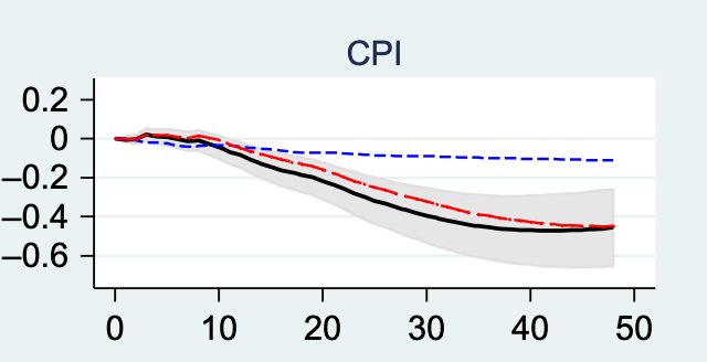
Fig. 1 Christiano et al. (1999) identification. 1965m1–1995m6 full specification: solid black lines; 1983m1–2007m12 full specification: short dashed blue (dark gray in the print version) lines; 1983m1–2007m12, omits money and reserves: long-dashed red (gray in the print version) lines. Light gray bands are 90% confidence bands. Source: Ramey 2016.  Months on x axis. 

The black lines plot the original specification. The top left panel plots the path of the Federal Funds rate after the Fed unexpectedly raises the interest rate. The funds rate goes up, but only for 6 months or so. Industrial production goes down and unemployment goes up, peaking at month 20. The figure plots the level of the CPI, so inflation is the slope of the lower right hand panel. You see inflation goes the "wrong" way, up, for about 6 months, and then gently declines. Interest rates indeed seem to affect the economy with long lags. 

This was the broad outline of consensus empirical estimates for many years. It is common to many other studies, and it is consistent with the beliefs of policy makers and analysts. It's pretty much what Friedman (1968) told us to expect. Getting contemporary models to produce something like this is much harder, but that's the next blog post. 

What's a VAR?

I try to keep this blog accessible to nonspecialists, so I'll step back momentarily to explain how we produce graphs like these. Economists who know what a VAR is should skip to the next section heading. 

How do we measure the effect of monetary policy on other variables? Milton Friedman and Anna Schwartz kicked it off in the Monetary History by pointing to the historical correlation of money growth with inflation and output. They knew as we do that correlation is not causation, so they pointed to the fact that money growth preceeded inflation and output growth.  But as James Tobin pointed out, the cock's crow comes before, but does not cause, the sun to rise. So too people may go get out some money ahead of time when they see more future business activity on the horizon.  Even correlation with a lead is not causation. What to do? Clive Granger's causality and Chris Sims' VAR, especially "Macroeconomics and Reality" gave today's answer. (And there is a reason that everybody mentioned so far has a Nobel prize.) 

First, we find a monetary policy "shock," a movement in the interest rate (these days; money, then) that is plausibly not a response to economic events and especially to expected future economic events. We think of the Fed setting interest rates by a response to economic data plus deviations from that response, such as

 interest rate = (#) output + (#) inflation + (#) other variables + disturbance. 

We want to isolate the "disturbance," movements in the interest rate not taken in response to economic events. (I use "shock" to mean an unpredictable variable, and "disturbance" to mean deviation from an equation like the above, but one that can persist for a while. A monetary policy "shock" is an unexpected movement in the disturbance.)  The "rule" part here can be but need not be the Taylor rule, and can include other variables than output and inflation. It is what the Fed usually does given other variables, and therefore (hopefully) controls for reverse causality from expected future economic events to interest rates. 

Now, in any individual episode, output and inflation and inflation following a shock will be influenced by subsequent shocks to the economy, monetary and other. But those average out. So, the average value of inflation, output, employment, etc. following a monetary policy shock is a measure of how the shock affects the economy all on its own. That is what has been plotted above. 

VARs were one of the first big advances in the modern empirical quest to find "exogenous" variation and (somewhat) credibly find causal relationships. 

Mostly the huge literature varies on how one finds the "shocks." Traditional VARs use regressions of the above equations and the residual is the shock, with a big question just how many and which contemporaneous variables one adds in the regression. Romer and Romer pioneered the "narrative approach," reading the Fed minutes to isolate shocks.  Some technical details at the bottom and much more discussion below. The key is finding shocks. One can just regress output and inflation on the shocks to produce the response function, which is a "local projection" not a "VAR," but I'll use "VAR" for both techniques for lack of a better encompassing word. 

Losing faith

• Shocks, what shocks?

What's a "shock" anyway? The concept is that the Fed considers its forecast of inflation, output and other variables it is trying to control, gauges the usual and appropriate response, and then adds 25 or 50 basis points, at random, just for the heck of it. The question VARS try to answer is the same: What happens to the economy if the Fed raises interest rates unexpectedly, for no particular reason at all? 

But the Fed never does this. Ask them. Read the minutes. The Fed does not roll dice. They always raise or lower interest rates for a reason, that reason is always a response to something going on in the economy, and most of the time how it affects forecasts of inflation and employment. There are no shocks as defined.

I speculated here that we might get around this problem: If we knew the Fed was responding to something that had no correlation with future output, then even though that is an endogenous response, then it is a valid movement for estimating the effect of interest rates on output. My example was, what if the Fed "responds" to the weather. Well, though endogenous, it's still valid for estimating the effect on output. 

The Fed does respond to lots of things, including foreign exchange, financial stability issues, equity, terrorist attacks, and so forth. But I can't think of any of these in which the Fed is not thinking of these events for their effect on output and inflation, which is why I never took the idea far. Maybe you can. 

Shock isolation also depends on complete controls for the Fed's information. If the Fed uses any information about future output and inflation that is not captured in our regression, then information about future output and inflation remains in the "shock" series. 

The famous "price puzzle" is a good example. For the first few decades of VARs, interest rate shocks seemed to lead to higher inflation. It took a long specification search to get rid of this undesired result. The story was, that the Fed saw inflation coming in ways not completely controlled for by the regression. The Fed raised interest rates to try to forestall the inflation, but was a bit hesitant about it so did not cure the inflation that was coming. We see higher interest rates followed by higher inflation, though the true causal effect of interest rates goes the other way. This problem was "cured" by adding commodity prices to the interest rate rule, on the idea that fast-moving commodity prices would capture the information the Fed was using to forecast inflation. (Interestingly these days we seem to see core inflation as the best forecaster, and throw out commodity prices!) With those and some careful orthogonalization choices, the "price puzzle" was tamped down to the one year or so delay you see above. (Neo-Fisherians might object that maybe the price puzzle was trying to tell us something all these years!) 

Nakamura and Steinsson write of this problem: 

"What is being assumed is that controlling for a few lags of a few variables captures all endogenous variation in policy... This seems highly unlikely to be true in practice. The Fed bases its policy decisions on a huge amount of data. Different considerations (in some cases highly idiosyncratic) affect policy at different times. These include stress in the banking system, sharp changes in commodity prices, a recent stock market crash, a financial crisis in emerging markets, terrorist attacks, temporary investment tax credits, and the Y2K computer glitch. The list goes on and on. Each of these considerations may only affect policy in a meaningful way on a small number of dates, and the number of such influences is so large that it is not feasible to include them all in a regression. But leaving any one of them out will result in a monetary policy “shock” that the researcher views as exogenous but is in fact endogenous." 

Nakamura and Steinsson offer 9/11 as another example summarizing my "high frequency identification" paper with Monika Piazzesi: The Fed lowered interest rates after the terrorist attack, likely reacting to its consequences for output and inflation. But VARs register the event as an exogenous shock.

Romer and Romer suggested that we use Fed Greenbook forecasts of inflation and output as controls, as those should represent the Fed's complete information set. They provide narrative evidence that Fed members trust Greenback forecasts more than you might suspect. 

This issue is a general Achilles heel of empirical macro and finance: Does your procedure assume agents see no more information than you have included in the model or estimate? If yes, you have a problem. Similarly, "Granger causality" answers the cock's crow-sunrise problem by saying that if unexpected x leads unexpected y then x causes y. But it's only real causality if the "expected" includes all information, as the price puzzle counterexample shows. 

Just what properties do we need of a shock in order to measure the response to the question, "what if the Fed raised rates for no reason?" This strikes me as a bit of an unsolved question -- or rather, one that everyone thinks is so obvious that we don't really look at it. My suggestion that the shock only need be orthogonal to the variable whose response we're estimating is informal, and I don't know of formal literature that's picked it up. 

Must "shocks" be unexpected, i.e. not forecastable from anything in the previous time information set? Must they surprise people? I don't think so -- it is neither necessary nor sufficient for  shock to be unforecastable for it to identify the inflation and output responses. Not responding to expected values of the variable whose response you want to measure should be enough.  If bond markets found out about a random funds rate rise one day ahead, it would then be an "expected" shock, but clearly just as good for macro. Romer and Romer have been criticized that their shocks are predictable, but this may not matter. 

The above Nakamura and Steinsson quote says leaving out any information leads to a shock that is not strictly exogenous. But strictly exogenous may not be necessary for estimating, say, the effect of interest rates on inflation. It is enough to rule out reverse causality and third effects. 

Either I'm missing a well known econometric literature, as is everyone else writing the VARs I've read who don't cite it, or there is a good theory paper to be written.

Romer and Romer, thinking deeply about how to read "shocks" from the Fed minutes, define shocks thus to circumvent the "there are no shocks" problem:

we look for times when monetary policymakers felt the economy was roughly at potential (or normal) output, but decided that the prevailing rate of inflation was too high. Policymakers then chose to cut money growth and raise interest rates, realizing that there would be (or at least could be) substantial negative consequences for aggregate output and unemployment. These criteria are designed to pick out times when policymakers essentially changed their tastes about the acceptable level of inflation. They weren’t just responding to anticipated movements in the real economy and inflation. 

[My emphasis.]  You can see the issue. This is not an "exogenous" movement in the funds rate. It is a response to inflation, and to expected inflation, with a clear eye on expected output as well. It really is a nonlinear rule, ignore inflation for a while until it gets really bad then finally get serious about it. Or, as they say, it is a change in rule, an increase in the sensitivity of the short run interest rate response to inflation, taken in response to inflation seeming to get out of control in a longer run sense. Does this identify the response to an "exogenous" interest rate increase? Not really.  But maybe it doesn't matter. 

• Are we even asking an interesting question? 

The whole question, what would happen if the Fed raised interest rates for no reason, is arguably besides the point. At a minimum, we should be clearer about what question we are asking, and whether the policies we analyze are implementations of that question. 

The question presumes a stable "rule," (e.g. \(i_t = \rho i_{t-1} + \phi_\pi \pi_t + \phi_x x_t + u_t\)) and asks what happens in response to a deviation \( +u_t \) from the rule. Is that an interesting question? The standard story for 1980-1982 is exactly not such an event. Inflation was not conquered by a big "shock," a big deviation from 1970s practice, while keeping that practice intact. Inflation was conquered (so the story goes) by a change in the rule, by a big increase in $\phi_\pi$. That change raised interest rates,  but arguably without any deviation from the new rule \(u_t\) at all. Thinking in terms of the Phillips curve \( \pi_t = E_t \pi_{t+1} + \kappa x_t\), it was not a big negative \(x_t\) that brought down inflation, but the credibility of the new rule that brought down \(E_t \pi_{t+1}\). 

If the art of reducing inflation is to convince people that a new regime has arrived, then the response to any monetary policy “shock” orthogonal to a stable “rule” completely misses that policy. 

Romer and Romer are almost talking about a rule-change event. For 2022, they might be looking at the Fed's abandonment of flexible average inflation targeting and its return to a Taylor rule. However, they don't recognize the importance of the distinction, treating changes in rule as equivalent to a residual. Changing the rule changes expectations in quite different ways from a residual of a stable rule. Changes with a bigger commitment should have bigger effects, and one should standardize somehow by the size and permanence of the rule change, not necessarily the size of the interest rate rise. And, having asked "what if the Fed changes rule to be more serious about inflation," we really cannot use the analysis to estimate what happens if the Fed shocks interest rates and does not change the rule. It takes some mighty invariance result from an economic theory that a change in rule has the same effect as a shock to a given rule. 

There is no right and wrong, really. We just need to be more careful about what question the empirical procedure asks, if we want to ask that question, and if our policy analysis actually asks the same question. 

• Estimating rules, Clarida Galí and Gertler. 

Clarida, Galí, and Gertler (2000) is a justly famous paper, and in this context for doing something totally different to evaluate monetary policy. They estimate rules, fancy versions of \(i_t = \rho i_{t-1} +\phi_\pi \pi_t + \phi_x x_t + u_t\), and they estimate how the \(\phi\) parameters change over time. They attribute the end of 1970s inflation to a change in the rule, a rise in \(\phi_\pi\) from the 1970s to the 1980s. In their model, a higher \( \phi_\pi\) results in less volatile inflation. They do not estimate any response functions. The rest of us were watching the wrong thing all along. Responses to shocks weren't the interesting quantity. Changes in the rule were the interesting quantity. 

Yes, I criticized the paper, but for issues that are irrelevant here. (In the new Keynesian model, the parameter that reduces inflation isn't the one they estimate.) The important point here is that they are doing something completely different, and offer us a roadmap for how else we might evaluate monetary policy if not by impulse-response functions to monetary policy shocks. 

• Fiscal theory

The interesting question for fiscal theory is, "What is the effect of an interest rate rise not accompanied by a change in fiscal policy?" What can the Fed do by itself? 

By contrast, standard models (both new and old Keynesian) include concurrent fiscal policy changes when interest rates rise. Governments tighten in present value terms, at least to pay higher interest costs on the debt and the windfall to bondholders that flows from unexpected disinflation. 

Experience and estimates surely include fiscal changes along with monetary tightening. Both fiscal and monetary authorities react to inflation with policy actions and reforms. Growth-oriented microeconomic reforms with fiscal consequences often follow as well -- rampant inflation may have had something to do with Carter era trucking, airline, and telecommunications reform. 

Yet no current estimate tries to look for a monetary shock orthogonal to fiscal policy change. The estimates we have are at best the effects of monetary policy together with whatever induced or coincident fiscal and microeconomic policy tends to happen at the same time as central banks get serious about fighting inflation. Identifying the component of a monetary policy shock orthogonal to fiscal policy, and measuring its effects is  a first order question for fiscal theory of monetary policy. That's why I wrote this blog post. I set out to do it, and then started to confront how VARs are already falling apart in our hands. 

Just what "no change in fiscal policy" means is an important question that varies by application. (Lots more in "fiscal roots" here, fiscal theory of monetary policy here and in FTPL.) For simple calculations, I just ask what happens if interest rates change with no change in primary surplus. One might also define "no change" as no change in tax rates, automatic stabilizers, or even habitual discretionary stimulus and bailout, no disturbance \(u_t\) in a fiscal rule \(s_t = a + \theta_\pi \pi_t + \theta_x x_t + ... + u_t\). There is no right and wrong here either, there is just making sure you ask an interesting question. 

• Long and variable lags, and persistent interest rate movements

The first plot shows a mighty long lag between the monitor policy shock and its effect on inflation and output. That does not mean that the economy has long and variable lags. 

This plot is actually not representative, because in the black lines the interest rate itself quickly reverts to zero. It is common to find a more protracted interest rate response to the shock, as shown in the red and blue lines. That mirrors common sense: When the Fed starts tightening, it sets off a year or so of stair-step further increases, and then a plateau, before similar stair-step reversion. 

That raises the question, does the long-delayed response of output and inflation represent a delayed response to the initial monetary policy shock, or does it represent a nearly instantaneous response to the higher subsequent interest rates that the shock sets off? 

Another way of putting the question, is the response of inflation and output invariant to changes in the response of the funds rate itself? Do persistent and transitory funds rate changes have the same responses? If you think of the inflation and output responses as economic responses to the initial shock only, then it does not matter if interest rates revert immediately to zero, or go on a 10 year binge following the initial shock. That seems like a pretty strong assumption. If you think that a more persistent interest rate response would lead to a larger or more persistent output and inflation response, then you think some of what we see in the VARs is a quick structural response to the later higher interest rates, when they come. 

Back in 1988, I posed this question in "what do the VARs mean?" and showed you can read it either way. The persistent output and inflation response can represent either long economic lags to the initial shock, or much less laggy responses to interest rates when they come. I showed how to deconvolute the response function to the structural effect of interest rates on inflation and output and how persistently interest rates rise.  The inflation and output responses might be the same with shorter funds rate responses, or they might be much different. 

Obviously (though often forgotten), whether the inflation and output responses are invariant to changes in the funds rate response needs a model. If in the economic model only unexpected interest rate movements affect output and inflation, though with lags, then the responses are as conventionally read structural responses and invariant to the interest rate path. There is no such economic model. Lucas (1972) says only unexpected money affects output, but with no lags, and expected money affects inflation. New Keynesian models have very different responses to permanent vs. transitory interest rate shocks. 

Interestingly, Romer and Romer do not see it this way, and regard their responses as structural long and variable lags, invariant to the interest rate response. They opine that given their reading of a positive shock in 2022, a long and variable lag to inflation reduction is baked in, no matter what the Fed does next. They argue that the Fed should stop raising interest rates. (In fairness, it doesn't look like they thought about the issue much, so this is an implicit rather than explicit assumption.) The alternative view is that effects of a shock on inflation are really effects of the subsequent rate rises on inflation, that the impulse response function to inflation is not invariant to the funds rate response, so stopping the standard tightening cycle would undo the inflation response. Argue either way, but at least recognize the important assumption behind the conclusions. 

Was the success of inflation reduction in the early 1980s just a long delayed response to the first few shocks? Or was the early 1980s the result of persistent large real interest rates following the initial shock? (Or, something else entirely, a coordinated fiscal-monetary reform... But I'm staying away from that and just discussing conventional narratives, not necessarily the right answer.) If the latter, which is the conventional narrative, then you think it does matter if the funds rate shock is followed by more funds rate rises (or positive deviations from a rule), that the output and inflation response functions do not directly measure long lags from the initial shock. De-convoluting the structural funds rate to inflation response and the persistent funds rate response, you would estimate much shorter structural lags. 

Nakamura and Steinsson are of this view: 

While the Volcker episode is consistent with a large amount of monetary nonneutrality, it seems less consistent with the commonly held view that monetary policy affects output with “long and variable lags.” To the contrary, what makes the Volcker episode potentially compelling is that output fell and rose largely in sync with the actions [interest rates, not shocks] of the Fed. 

And that's a good thing too. We've done a lot of dynamic economics since Friedman's 1968 address. There is really nothing in dynamic economic theory that produces a structural long-delayed response to shocks, without the continued pressure of high interest rates. (A correspondent objects to "largely in sync" pointing out several clear months long lags between policy actions and results in 1980. It's here for the methodological point, not the historical one.) 

However, if the output and inflation responses are not invariant to the interest rate response, then the VAR directly measures an incredibly narrow experiment: What happens in response to a surprise interest rate rise, followed by the plotted path of interest rates? And that plotted path is usually pretty temporary, as in the above graph. What would happen if the Fed raised rates and kept them up, a la 1980? The VAR is silent on that question. You need to calibrate some model to the responses we have to infer that answer. 

VARs and shock responses are often misread as generic theory-free estimates of "the effects of monetary policy." They are not. At best, they tell you the effect of one specific experiment: A random increase in funds rate, on top of a stable rule, followed by the usual following path of funds rate. Any other implication requires a model, explicit or implicit. 

More specifically, without that clearly false invariance assumption, VARs cannot directly answer a host of important questions. Two on my mind: 1) What happens if the Fed raises interest rates permanently? Does inflation eventually rise? Does it rise in the short run? This is the "Fisherian" and "neo-Fisherian" questions, and the answer "yes" pops unexpectedly out of the standard new-Keynesian model. 2) Is the short-run negative response of inflation to interest rates stronger for more persistent rate rises? The long-term debt fiscal theory mechanism for a short-term inflation decline is tied to the persistence of the shock and the maturity structure of the debt. The responses to short-lived interest rate movements (top left panel) are silent on these questions. 

Directly is an important qualifier. It is not impossible to answer these questions, but you have to work harder to identify persistent interest rate shocks. For example, Martín Uribe identifies permanent vs. transitory interest rate shocks, and finds a positive response of inflation to permanent interest rate rises. How? You can't just pick out the interest rate rises that turned out to be permanent. You have to find shocks or components of the shock that are ex-ante predictably going to be permanent, based on other forecasting variables and the correlation of the shock with other shocks. For example, a short-term rate shock that also moves long-term rates might be more permanent than one which does not do so. (That requires the expectations hypothesis, which doesn't work, and long term interest rates move too much anyway in response to transitory funds rate shocks. So, this is not directly a suggestion, just an example of the kind of thing one must do. Uribe's model is more complex than I can summarize in a blog.)  Given how small and ephemeral the shocks are already, subdividing them into those that are expected to have permanent vs. transitory effects on the federal funds rate is obviously a challenge. But it's not impossible. 

• Monetary policy shocks account for small fractions of inflation, output and funds rate variation. 

Friedman thought that most recessions and inflations were due to monetary mistakes. The VARs pretty uniformly deny that result. The effects of monetary policy shocks on output and inflation add up to less than 10 percent of the variation of output and inflation. In part the shocks are small, and in part the responses to the shocks are small. Most recessions come from other shocks, not monetary mistakes.  

Worse, both in data and in models, most inflation variation comes from inflation shocks, most output variation comes from output shocks, etc. The cross-effects of one variable on another are small. And "inflation shock" (or "marginal cost shock"),  "output shock" and so forth are just labels for our ignorance -- error terms in regressions, unforecasted movements -- not independently measured quantities. 

(This and old point, for example in my 1994 paper with the great title "Shocks." Technically, the variance of output is the sum of the squares of the impulse-response functions -- the plots -- times the variance of the shocks. Thus small shocks and small responses mean not much variance explained.)

This is a deep point. The exquisite attention put to the effects of monetary policy in new-Keynesian models, while interesting to the Fed, are then largely beside the point if your question is what causes recessions. Comprehensive models work hard to match all of the responses, not just to monetary policy shocks. But it's not clear that the nominal rigidities that are important for the effects of monetary policy are deeply important to other (supply) shocks, and vice versa. 

This is not a criticism. Economics always works better if we can use small models that focus on one thing -- growth, recessions, distorting effect of taxes, effect of monetary policy -- without having to have a model of everything in which all effects interact. But, be clear we no longer have a model of everything.  "Explaining recessions" and "understanding the effects of monetary policy" are somewhat separate questions. 

Monetary policy shocks also account for small fractions of the movement in the federal funds rate itself. Most of the funds rate movement is in the rule, the reaction to the economy term. Like much empirical economics, the quest for causal identification leads us to look at a tiny causes with tiny effects, that do little to explain much variation in the variable of interest (inflation). Well, cause is cause, and the needle is the sharpest item in the haystack. But one worries about the robustness of such tiny effects, and to what extent they summarize historical experience.  

To be concrete, here is a typical shock regression, 1960:1-2023:6 monthly data, standard errors in parentheses: 

ff(t) = a + b ff(t-1) + c[ff(t-1)-ff(t-2)] + d CPI(t) + e unemployment(t) + monetary policy shock, 

Where "CPI" is the percent change in the CPI (CPIAUCSL) from a year earlier. 

ff(t-1)	ff(t-1)-ff(t-2)	CPI	Unemp	R2
0.97	0.39	0.032	-0.017	0.985
(0.009)	(0.07)	(0.013)	(0.009)

The funds rate is persistent -- the lag term (0.97) is large. Recent changes matter too: Once the Fed starts a tightening cycle, it's likely to keep raising rates. And the Fed responds to CPI and unemployment. 

The plot shows the actual federal funds rate (blue), the model or predicted federal funds rate (red), the shock which is the difference between the two (orange) and the Romer and Romer dates (vertical lines). You can't see the difference between actual and predicted funds rate, which is the point. They are very similar and the shocks are small. They are closer horizontally than vertically, so the vertical difference plotted as shock is still visible. 

The shocks are much smaller than the funds rate, and smaller than the rise and fall in the funds rate in a typical tightening or loosening cycle. The shocks are bunched, with by far the biggest ones in the early 1980s. The shocks have been tiny since the 1980s. (Romer and Romer don't find any shocks!) 

Now, our estimates of the effect of monetary policy look at the average values of inflation, output, and employment in the 4-5 years after a shock. Really, you say, looking at the graph? That's going to be dominated by the experience of the early 1980s. And with so many positive and negative shocks close together, the average value 4 years later is going to be driven by subtle timing of when the positive or negative shocks line up with later events. 

Put another way, here is a plot of inflation 30 months after a shock regressed on the shock. Shock on the x axis, subsequent inflation on the y axis. The slope of the line  is our estimate of the effect of the shock on inflation 30 months out (source, with details). Hmm. 

One more graph (I'm having fun here):

This is a plot of inflation for the 4 years after each shock, times that shock. The right hand side is the same graph with an expanded y scale. The average of these histories is our impulse response function.  (The big lines are the episodes which multiply the big shocks of the early 1980s. They mostly converge because, either multiplied by positive or negative shocks, inflation wend down in the 1980s.) 

Impulse response functions are just quantitative summaries of the lessons of history. You may be  underwhelmed that history is sending a clear story.  

Again, welcome to causal economics -- tiny average responses to tiny but identified movements is what we estimate, not broad lessons of history. We do not estimate "what is the effect of the sustained high real interest rates of the early 1980s," for example, or "what accounts for the sharp decline of inflation in the early 1980s?" Perhaps we should, though confronting endogeneity of the interest rate responses some other way. That's my main point today. 

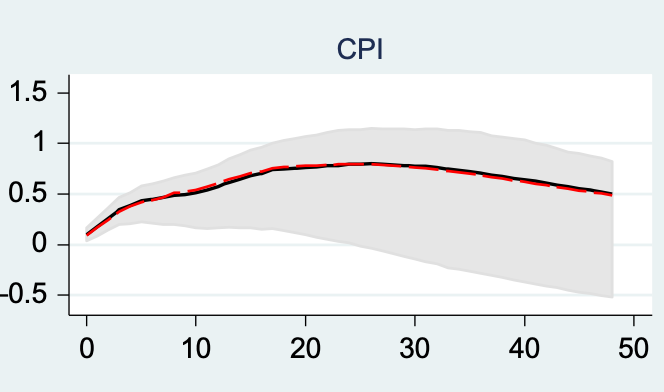
• Estimates disappear after 1982

Ramey's first variation in the first plot is to use data from 1983 to 2007. Her second variation is to also omit the monetary variables. Christiano Eichenbaum and Evans were still thinking in terms of money supply control, but our Fed does not control money supply. 

The evidence that higher interest rates lower inflation disappears after 1983, with or without money. This too is a common finding. It might be because there simply aren't any monetary policy shocks. Still, we're driving a car with a yellowed AAA road map dated 1982 on it.  

Monetary policy shocks still seem to affect output and employment, just not inflation. That poses a deeper problem. If there just aren't any monetary policy shocks, we would just get big standard errors on everything. That only inflation disappears points to the vanishing Phillips curve, which will be the weak point in the theory to come. It is the Phillips curve by which lower output and employment push down inflation. But without the Phillips curve, the whole standard story for interest rates to affect inflation goes away. 

• Computing long-run responses

The long lags of the above plot are already pretty long horizons, with interesting economics still going on at 48 months. As we get interested in long run neutrality, identification via long run sign restrictions (monetary policy should not permanently affect output), and the effect of persistent interest rate shocks, we are interested in even longer run responses. The "long run risks" literature in asset pricing is similarly crucially interested in long run properties. Intuitively, we should know this will be troublesome. There aren't all that many nonoverlapping 4 year periods after interest rate shocks to measure effects, let alone 10 year periods.

VARs estimate long run responses with a parametric structure. Organize the data (output, inflation, interest rate, etc) into a vector \(x_t = [y_t \; \pi_t \; i_t \; ...]'\), then the VAR can be written \(x_{t+1} = Ax_t + u_t\). We start from zero, move \(x_1 = u_1\) in an interesting way, and then the response function just simulates forward, with \(x_j = A^j x_1\).  

But here an oft-forgotten lesson of 1980s econometrics pops up: It is dangerous to estimate long-run dynamics by fitting a short run model and then finding its long-run implications. Raising matrices to the 48th power \(A^{48}\) can do weird things, the 120th power (10 years) weirder things. OLS and maximum likelihood prize one step ahead \(R^2\), and will happily accept small one step ahead mis specifications that add up to big misspecification 10 years out. (I learned this lesson in the "Random walk in GNP.") 

Long run implications are driven by the maximum eigenvalue of the \(A\) transition matrix, and its associated eigenvector. \(A^j = Q \Lambda^j Q^{-1}\).  This is a benefit and a danger. Specify and estimate the dynamics of the combination of variables with the largest eigenvector  right, and lots of details can be wrong. But standard estimates aren't trying hard to get these right. 

The "local projection" alternative directly estimates long run responses: Run regressions of inflation in 10 years on the shock today. You can see the tradeoff: there aren't many non-overlapping 10 year intervals, so this will be imprecisely estimated. The VAR makes a strong parametric assumption about long-run dynamics. When it's right, you get better estimates. When it's wrong, you get misspecification. 

My experience running lots of VARs is that monthly VARs raised to large powers often give unreliable responses. Run at least a one-year VAR before you start looking at long run responses. Cointegrating vectors are the most reliable variables to include. They are typically the state variable that most reliably carries long - run responses. But pay attention to getting them right. Imposing integrating and cointegrating structure by just looking at units is a good idea. 

The regression of long-run returns on dividend yields is a good example. The dividend yield is a cointegrating vector, and is the slow-moving state variable. A one period VAR \[\left[ \begin{array}{c} r_{t+1} \\ dp_{t+1} \end{array} \right] = \left[ \begin{array}{cc} 0 & b_r  \\ 0 & \rho \end{array}\right]    \left[ \begin{array}{c} r_{t} \\ dp_{t} \end{array}\right]+ \varepsilon_{t+1}\] implies a long horizon regression \(r_{t+j} = b_r \rho^j dp_{t} +\) error. Direct regressions ("local projections") \(r_{t+j} = b_{r,j} dp_t + \) error give about the same answers, though the downward bias in \(\rho\) estimates is a bit of an issue, but with much larger standard errors. The constraint \(b_{r,j} = b_r \rho^j\) isn't bad. But it can easily go wrong. If you don't impose that dividends and price are cointegrated, or with vector other than 1 -1, if you  allow a small sample to estimate \(\rho>1\), if you don't put in dividend yields at all and just a lot of short-run forecasters, it can all go badly. 

Forecasting bond returns was for me a good counterexample. A VAR forecasting one-year bond returns  from today's yields gives very different results from taking a monthly VAR, even with several lags, and using \(A^{12}\) to infer the one-year return forecast. Small pricing errors or microstructure dominate the monthly data, which produces junk when raised to the twelfth power. (Climate regressions are having fun with the same issue. Small estimated effects of temperature on growth, raised to the 100th power, can produce nicely calamitous results. But use basic theory to think about units.)  

Nakamura and Steinsson (appendix) show how sensitive some standard estimates of impulse response functions are to these questions. 

Weak evidence

For the current policy question, I hope you get a sense of how weak the evidence is for the "standard view" that higher interest rates reliably lower inflation, though with a long and variable lag, and the Fed has a good deal of control over inflation. 

Yes, many estimates look the same, but there is a pretty strong prior going in to that. Most people don't publish papers that don't conform to something like the standard view. Look how long it took from Sims (1980) to Christiano Eichenbaum and Evans (1999) to produce a response function that does conform to the standard view, what Friedman told us to expect in (1968). That took a lot of playing with different orthogonalization, variable inclusion, and other specification assumptions. This is not criticism: when you have a strong prior, it makes sense to see if the data can be squeezed in to the prior. Once authors like Ramey and Nakamura and Steinsson started to look with a critical eye, it became clearer just how weak the evidence is. 

Standard errors are also wide, but the variability in results due to changes in sample and specification are much larger than formal standard errors. That's why I don't stress that statistical aspect. You play with 100 models, try one variable after another to tamp down the price puzzle, and then compute standard errors as if the 100th model were written in stone. This post is already too long, but showing how results change with different specifications would have been a good addition. 

For example, here are a few more Ramey plots of inflation responses, replicating various previous estimates

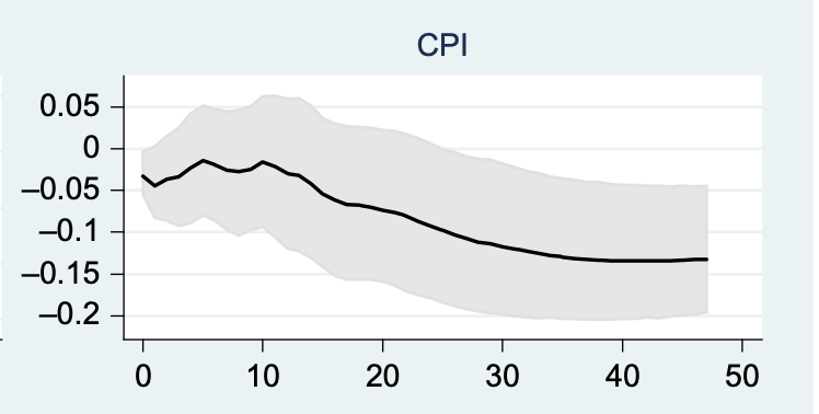
Take your pick. 

What should we do instead? 

Well, how else should we measure the effects of monetary policy? One natural approach turns to the analysis of historical episodes and changes in regime, with specific models in mind. 

Romer and Romer pass on thoughts on this approach: 

...some macroeconomic behavior may be fundamentally episodic in nature. Financial crises, recessions, disinflations, are all events that seem to play out in an identifiable pattern. There may be long periods where things are basically fine, that are then interrupted by short periods when they are not. If this is true, the best way to understand them may be to focus on episodes—not a cross-section proxy or a tiny sub-period. In addition, it is valuable to know when the episodes were and what happened during them. And, the identification and understanding of episodes may require using sources other than conventional data.

A lot of my and others'  fiscal theory writing has taken a similar view. The long quiet zero bound is a test of theories: old-Keynesian models predict a delation spiral, new-Keynesian models predicts sunspot volatility, fiscal theory is consistent with stable quiet inflation.  The emergence of inflation in 2021 and its easing despite interest rates below inflation likewise validates fiscal vs. standard theories.  The fiscal implications of abandoning the gold standard in 1933 plus Roosevelt's "emergency" budget make sense of that episode. The new-Keynesian reaction parameter \(\phi_\pi\) in \(i_t - \phi_\pi \pi_t\), which leads to unstable dynamics for ](\phi_\pi>1\) is not identified by time series data. So use "other sources," like plain statements on the Fed website about how they react to inflation. I already cited Clarida Galí and Gertler, for measuring the rule not the response to the shock, and explaining the implications of that rule for their model. 

Nakamura and Steinsson likewise summarize Mussa's (1986) classic study of what happens when countries switch from fixed to floating exchange rates: 

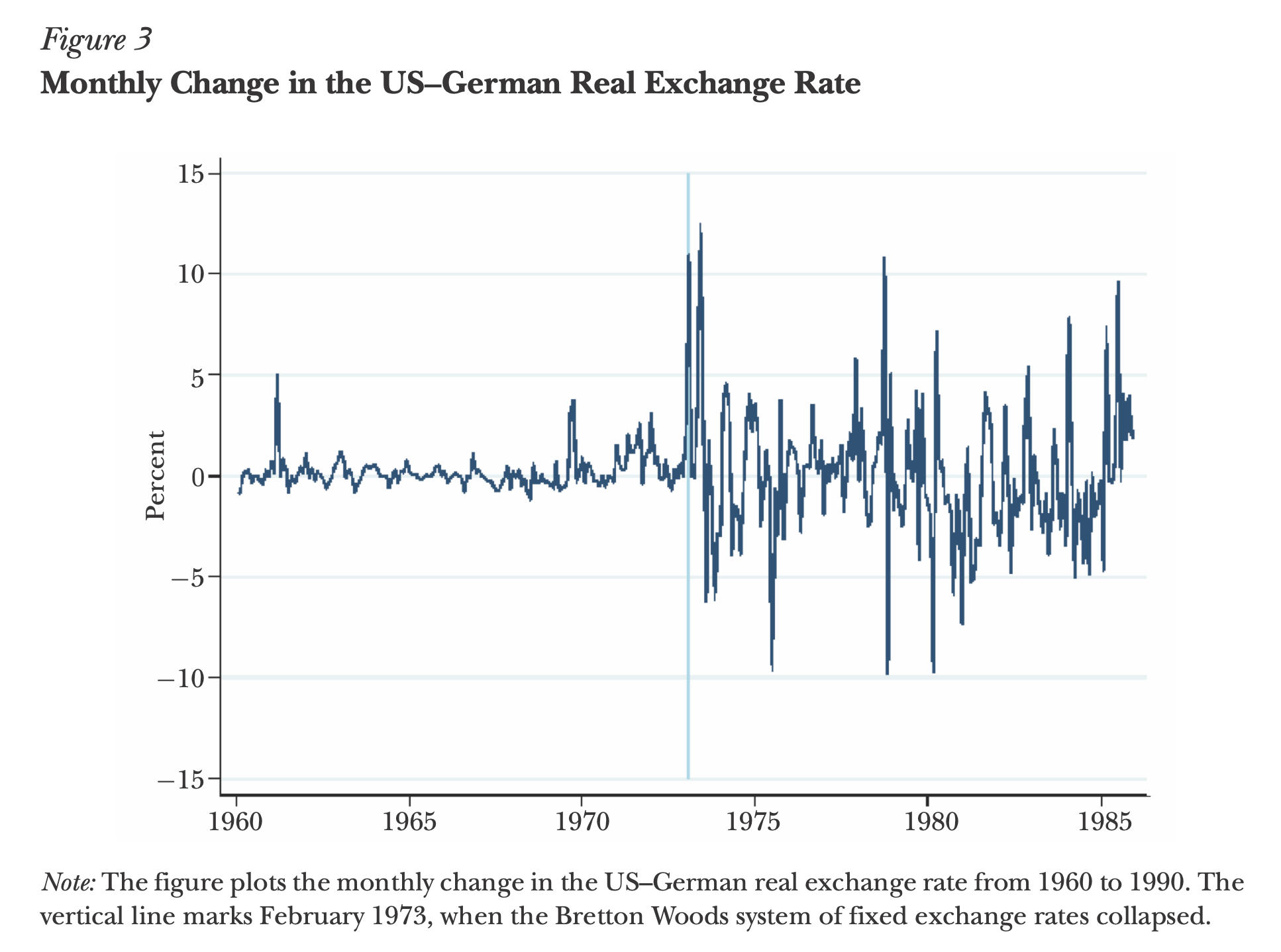
"The switch from a fixed to a flexible exchange rate is a purely monetary action. In a world where monetary policy has no real effects, such a policy change would not affect real variables like the real exchange rate. Figure 3 demonstrates dramatically that the world we live in is not such a world."

Also, analysis of particular historical episodes is enlightening. But each episode has other things going on and so invites alternative explanations. 90 years later, we're still fighting about what caused the Great Depression. 1980 is the poster child for monetary disinflation, yet as Nakamura and Steinsson write, 

Many economists find the narrative account above and the accompanying evidence about output to be compelling evidence of large monetary nonneutrality. However, there are other possible explanations for these movements in output. There were oil shocks both in September 1979 and in February 1981.... Credit controls were instituted between March and July of 1980. Anticipation effects associated with the phased-in tax cuts of the Reagan administration may also have played a role in the 1981–1982 recession ....

Studying changes in regime, such as fixed to floating or the zero bound era, help somewhat relative to studying a particular episode, in that they have some of the averaging of other shocks. 

But the attraction of VARs will remain. None of these produces what VARs seemed to produce, a theory-free qualitative estimate of the effects of monetary policy. Many tell you that prices are sticky, but not how prices are sticky. Are they old-Keynesian backward looking sticky or new-Keynesian rational expectations sticky? What is the dynamic response of relative inflation to a change in a pegged exchange rate? What is the dynamic response of real relative prices to productivity shocks? Observations such as Mussa's graph can help to calibrate models, but does not answer those questions directly.  My observations about the zero bound or the recent inflation similarly seem (to me) decisive about one class of model vs. another, at least subject to Occam's razor about epicycles, but likewise do not provide a theory-free  impulse response function.  Nakamura and Steinsson write at length about other approaches; model-based moment matching and use of micro data in particular. This post is going on too long; read their paper. 

Of course, as we have seen, VARs only seem to offer a model-free quantitative measurement of "the effects of monetary policy," but it's hard to give up on the appearance of such an answer. VARs and impulse responses also  remain very useful ways of summarizing the correlations and cross correlations of data, even without cause and effect interpretation. 

In the end, many ideas are successful in economics when they tell researchers what to do, when they offer a relatively clear recipe for writing papers. "Look at episodes and think hard is not such  recipe." "Run a VAR is." So, as you think about how we can evaluate monetary policy, think about a better recipe as well as a good answer.  

(Stay tuned. This post is likely to be updated a few times!) 

VAR technical appendix

Technically, running VARs is very easy, at least until you start trying to smooth out responses with Bayesian  and other techniques. Line up the data in a vector, i.e. \(x_t = [i_t \; \pi_t\; y_t]'\). Then run a regression of each variable on lags of the others, \[x_t = Ax_{t-1} + u_t.\] If you want more than one lag of the right hand variables, just make a bigger \(x\) vector,  \(x_t = [i_t\; \pi_t \; y_t \; i_{t-1}\; \pi_{t-1} \;y_{t-1}]'.\) 

The residuals of such regressions \(u_t\) will be correlated, so you have to decide whether, say, the correlation between interest rate and inflation shocks means the Fed responds in the period to inflation, or inflation responds within the period to interest rates, or some combination of the two. That's the  "identification" assumption issue. You can write it as a matrix \(C\) so that \(u_t = C \varepsilon_t\) and cov\((\varepsilon_t \varepsilon_t')=I\) or you can include some contemporaneous values into the right hand sides. 

Now, with \(x_t = Ax_{t-1} + C\varepsilon_t\), you start with \(x_0=0\), choose one series to shock, e.g. \(\varepsilon_{i,1}=1\) leaving the others alone, and just simulate forward. The resulting path of the other variables is the above plot, the "impulse response function." Alternatively you can run a regression \(x_t = \sum_{j=0}^\infty \theta_j \varepsilon_{t-j}\) and the \(\theta_j\) are (different, in sample) estimates of the same thing. That's "local projection". Since the right hand variables are all orthogonal, you can run single or multiple regressions. (See here for equations.) Either way, you have found the moving average representation, \(x_t = \theta(L)\varepsilon_t\), in the first case with \(\theta(L)=(I-AL)^{-1}C\) in the second case directly. Since the right hand variables are all orthogonal, the variance of the series is the sum of its loading on all of the shocks, \(cov(x_t) = \sum_{j=0}^\infty \theta_j \theta_j'\). This "forecast error variance decomposition" is behind my statement that small amounts of inflation variance are due to monetary policy shocks rather than shocks to other variables, and mostly inflation shocks.   

Update:

Luis Garicano has a great tweet thread explaining the ideas with a medical analogy. Kamil Kovar has a nice follow up blog post, with emphasis on Europe. 

He makes a good point that I should have thought of: A monetary policy "shock" is a deviation from a "rule." So, the Fed's and ECB's failure to respond to inflation as they "usually" do in 2021-2022 counts exactly the same as a 3-5% deliberate lowering of the interest rate. Lowering interest rates for no reason, and leaving interest rates alone when the regression rule says raise rates are the same in this methodology.  That "loosening" of policy was quickly followed by inflation easing, so an updated VAR should exhibit a strong "price puzzle" -- a negative shock is followed by less, not more inflation. Of course historians and practical people might object that failure to act as usual has exactly the same effects as acting. 

* Some Papers: 

Comment on Romer and Romer What ends recessions? Some "what's a shock?"

Comment on Romer and Romer A new measure of monetary policy. The greenbook forecasts, and beginning thoughts that strict exogeneity is not necessary. 

Shocks monetary shocks explain small fractions of output variance.

Comments on Hamilton, more thoughts on what a shock is.

What do the VARs mean? cited above, is the response to the shock or to persistent interest rates?

The Fed and Interest Rates, with Monika Piazzesi. Daily data and interest rates to identify shocks. 

Decomposing the yield curve with Monika Piazzesi. Starts with a  great example of how small changes in specification lead to big differences in long run forecasts. 

Time series

A critique of the application of unit root tests pretesting for unit roots and cointegration is a bad idea

How big is the random walk in GNP? lessons in not using short run dynamics to infer long run properties. 

Permanent and transitory components of GNP and stock prices a favorite of cointegration really helps on long run properties

Time series for macroeconomics and finance notes that never quite became a book. Explains VARs and responses.